DMFTpack

DMFTpack is the software for DFT+DMFT calculation. Various projection methods [1] and the impurity solvers are available, e.g., iterative perturbation theory (IPT), self-consistent second-order perturbation theory (SC2PT). The interface connecting DFT package, e.g., OpenMX and impurity solvers (CT-QMC) is also provided.

Developer: Jae-Hoon Sim (email: jhsim4279@gmail.com)

Download

DMFTpack.tar.gz

Requirements

Impurity solver

(Optional) Hybridization expansion quantum Monte Carlo impurity solver: [To perform the CT-QMC solver, one of the following solvers should be installed: Otherwise, one can use the (SC) 2PT solver, which is implemented in the DMFTpack itself.]
- Implemented in ALPS library http://alps.comp-phys.org
- Implemented by K. Haule at Rutgers University http://www.physics.rutgers.edu/~haule/ (See also to install impurity solver: link)

Eigen (>=3.3)

C++ template library for linear algebra: matrices, vectors, numerical solvers, and related algorithms. http://eigen.tuxfamily.org
Since Eigen version 3.3 or later, you can use the BLAS / LAPACK or Intel MKL libraries.
- Using BLAS/LAPACK from Eigen http://eigen.tuxfamily.org/dox/TopicUsingBlasLapack.html
- Using Intel® MKL from Eigen http://eigen.tuxfamily.org/dox/TopicUsingIntelMKL.html

Installation

Install pre-requirements. Note that the LAPACK or Intel MKL libraries are optional:

$ sudo apt-get install gcc g++
$ sudo apt install openmpi-common openmpi-bin libopenmpi-dev
$ sudo apt install make
$ sudo apt-get install liblapack-dev

Install Eigen library:

$ git clone https://github.com/eigenteam/eigen-git-mirror

Install DMFTpack code:

$ git clone https://github.com/ElectronicStructureTheory-KAIST/DMFTinOpenMX_dev.git
$ cd DMFTinOpenMX_dev/src
$ vi makefile  (Replace the variables with ${} to the proper values for your system.)
$ make all

(Optional) Install MQEM to perform the analytic continuation:

$ git clone https://github.com/ElectronicStructureTheory-KAIST/MQEM.git

Example

Hubbard model

Test calculation can be performed for single-band Hubbard model as following:

$ cd ../example/Hubb_model/primitive_Cell_ipt
$ mpirun -np 4 ../../dmft | tee "std.out"
$ gnuplot gw_loc_Im.gnuplot
$ gnuplot sw_Im.gnuplot

Now, one may want to do analytic continuation from the Matsubara Green’s function (or the Self-energy) to the real-frequency spectral function.
```
$ mkdir realFreqSpectrum; cd realFreqSpectrum
$ mkdir continuation; cd continuation
```
- Any continuation method can be used to obtain the density of states from the Green’s function, e.g., MQEM (PRB 98, 205102 (2018))
```
$ cp ../../Sw_SOLVER.full.dat  ./
$ julia $(MQEM_dir)/src/mem.jl Sw_SOLVER.full.dat ../../input.solver | tee "std.out"
```
  or ΩMaxent (PRE 94, 023303 (2016)).
```
$ cp ../../Sw_SOLVER.dat  ./
$ ~/bin/OmegaMaxEnt | tee "std.out"
```
- For the case of self-energy continuation, one may want to generate “realFreq_Sw.dat_i_j” files, using the Kramers-Kronig relation. Here i and j are orbital indices. Each file contains omega for the first column and real and imaginary part of the self-energy for the second and third column, respectively.
- (optional) For the system with large spin-orbit coupling, we recommend MQEM method developed by J.-H. Sim [2]. The source code will be available soon via GitHub (update: 2018-10-19).
  - mqem.input.toml file is generated, one can control parameters for MQEM continuation method as following (See https://github.com/KAIST-ELST/MQEM.jl for more details):
  - (key) = (variable)

band structure: To do calculate band structure, SOLVER_TYPE=TB and RESTART>1 in input.pam is required, providing “realFreq_Sw.dat_i_j”.

$ mkdir ../bandstruc; cd ../bandstruc
$ cp  -r ../continuation/realFreq_Sw.dat_*  ../../Inputfiles/*  ../../Restart   ./
$ vi input.parm
$ mpirun -np 4 ../../../../dmft | tee "std.out"

Now one can plot the band structure as following:
```
$ python qsband.plot.py
```

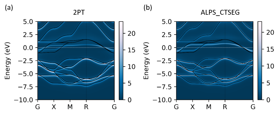
SrVO3

As same way, one can obtain band structure of the SrVO3 .
For DFT+DMFT calculation, non-interacting Hamiltonian is written in “SYSTEM_NAME.scfout” file, which is the output of the OpenMX code. (In this example one can simply uncompress “SVO113.tar.xz” file)
The figure below shows that the SrVO3 Band structure, calculated by two different impurity solvers, namely 2PT and ALPS_CTSEG.

Document

list of input parameters

After running OpenMX with option “ HS.fileout on”, two additional input files required for DMFT calculation.

List of input files
- “input.parm”: the computational information is written here. See below for more details.
- “input.solver”: information for impurity solver, e.g., U, N_TAU, …
- “SYSTEM_NAME.scfout”, which can be obtained from OpenMX code output.
  
  Alternatively, “SYSTEM_NAME.scfout” will be replaced by “Hk.HWR” and “OverlapMatrix.HWR”(optional): non-interacting Hamiltonian is written in the “Hk.HWR” file. When the non-orthogonal basis is used, the overlap matrix should be provided.
input.parm
- Computational information:
  - SYSTEM_NAME
  - SOLVER_TYPE = {ALPS_CTSEG, RUTGERS_CTSET, RUTGERS_CTHYB, IPT, SC2PT, 2PT, TB}
  - SOLVER_DIR = path to impurity solver (default: ~/bin/)
  - SOLVER_EXE = executable impurity solver (default: hybridization)
  - MAX_DMFT_ITER ={1,2…}, maximum DMFT iteration (default: 20)
  - MIXING = (default: 0.8), self-energy mixing weight in the DMFT iteration
  - RESTART = {0,1,…}, for initial calculation, >0 to start self-energy obtained from previous calculation. (default: 0)
- Lattice information
  - N_ATOMS = {1,2,..}, the number of atoms in the unit cell
  - N_CORRELATED_ATOMS = {1,2,…}, the number of atoms containing strong correlated orbitals.
  - N_ELECTRONS = {1,2,…} total number of the electrons in the unit cell.
  - MAGNETISM = {0,1,[2]} (default: 2)
  - K_POINTS = (nk1,nk2,nk3) k-grids to discretize the first Brillouin zone.
- DFT+DMFT option
  - H0_FROM_OPENMX = {0,1} = 1 if “SYSTEM_NAME”.scfout file is exist. Otherwise, Hk.HWR file should b exist in the work folder with “H0_FROM_OPENMX”=0.
  - num_subshell = the number of nl subshell for each orbital, e.g., num_subshell=5 for s2p2d1 basis
  - rot_sym = Quantum number l of the angular momentum for each subshell.
  - subshell = dimension of the subshell.
  - Rydberg_set = 0 for nominally occupied orbitals, 1 for empty
- Projection method We provide a method to obtain projective Wannier functions based on the natural atomic orbitals. The basic idea of the method is introduced in Ref. 1.
  - MODEL_WINDOW_U = upper bound of the energy window for the correlated subspace. The correlated orbitals are projected into the model window (default: 10).
  - MODEL_WINDOW_D = lower bound of the energy window for the correlated subspace (default: -10)
  - DC_TYPE = {nominal, [fll]}, double counting method (default: fll)
  - N_d = {0,1,..}, nominal charge in the correlated orbitals
  - HARTREE_ATOMS = {1,2,…} Atom indices of the correlated atoms
  - HARTREE_ORBITALS_RANGE = the range of the correlated orbitals indices
- DOS & Band calculation
  - MODE = {band, qsband, dos, qsband}, specifies the band/dos calculation for non-interacting (or quasi-particle) dispersion
  - K_GRID_BAND = (default: 40)
  - SPECTRAL_ENERGY_GRID = (default: 1000)
  - N_K_PATH = the number of paths for the band calculation
- K_PATH = this keword specifies the paths of the band dispersion
input.solver
- impurity_information
  - N_ORBITALS = the number of orbitals in impurity site
  - N_HARTREE_ORBITALS = the number of the correlated orbitals
  - U = intra-orbital interaction
  - U’ = inter-orbital interaction
  - J = Hund’s coupling
  - BETA = inverse temperature
- Matsubara_frequency
  - N_MATSUBARA = the number of the Matsubara frequencies
  - N_TAU = mesh grids in the imaginary time axis
- ALPS_CT_HYB_input
  - MEASURE_legendre = should be choose “1”
  - MEASURE_freq = should be choose “1”
  - TEXT_OUTPUT = should be choose “1”
  - MU_VECTOR = should be set as “mu_vector.alps.dat”
  - DELTA = should be set as “delta_t.dat”

Useful output files

Gw_loc.full.dat[N]: Local Green’s function G_αβ(iω_n) for N-th correlated atom. For each line, five numbers represent the n, α, β, real and imaginary part of the Green’s function, respectively.
Gw_imp.full.dat[N]: Same for impurity Green’s function.
Sw_SOLVER.full.dat: Self-energy calculated from the impurity solver.
Numele.dat: Number matrix n_αβ calculated by -G_αβ(τ=β^-).

References

DFT+DMFT with natural atomic orbital projectors Jae-Hoon Sim and Myung Joon Han, (Submitted)
Maximum Quantum Entropy Method Jae-Hoon Sim and Myung Joon Han, Phys. Rev. B 98, 205102 (2018)